Guided mode expansion with Autograd

import numpy as np
import matplotlib.pyplot as plt
import time

import autograd.numpy as npa
from autograd import grad, value_and_grad

import legume
from legume.minimize import Minimize

%load_ext autoreload
%autoreload 2

The autoreload extension is already loaded. To reload it, use:
  %reload_ext autoreload

PhC cavity simulation

In this Notebook, we will optimize a photonic crystal cavity in a lithium niobate slab. We use the small-volume design of Minkov et al., APL 111 (2017), and optimize with respect to shifts in the positions of the air holes. So, we start by defining the starting structure, and a function that builds the photonic crystal given some hole shifts. The PhC parameters are as from Li et al., https://arxiv.org/abs/1806.04755

# Number of PhC periods in x and y directions
Nx, Ny = 16, 10

# Regular PhC parameters
ra = 0.234
dslab = 0.4355
n_slab = 2.21

# Initialize a lattice and PhC
lattice = legume.Lattice([Nx, 0], [0, Ny*np.sqrt(3)/2])

# Make x and y positions in one quadrant of the supercell
# We only initialize one quadrant because we want to shift the holes symmetrically
xp, yp = [], []
nx, ny = Nx//2 + 1, Ny//2 + 1
for iy in range(ny):
    for ix in range(nx):
        xp.append(ix + (iy%2)*0.5)
        yp.append(iy*np.sqrt(3)/2)

# Move the first two holes to create the L4/3 defect
xp[0] = 2/5
xp[1] = 6/5
nc = len(xp)

# Initialize shift parameters to zeros
dx, dy = np.zeros((nc,)), np.zeros((nc,))

# Define L4/3 PhC cavity with shifted holes
def cavity(dx, dy):
    # Initialize PhC
    phc = legume.PhotCryst(lattice)

    # Add a layer to the PhC
    phc.add_layer(d=dslab, eps_b=n_slab**2)

    # Apply holes symmetrically in the four quadrants
    for ic, x in enumerate(xp):
        yc = yp[ic] if yp[ic] == 0 else yp[ic] + dy[ic]
        xc = x if x == 0 else xp[ic] + dx[ic]
        phc.add_shape(legume.Circle(x_cent=xc, y_cent=yc, r=ra))
        if nx-0.6 > xp[ic] > 0 and (ny-1.1)*np.sqrt(3)/2 > yp[ic] > 0:
            phc.add_shape(legume.Circle(x_cent=-xc, y_cent=-yc, r=ra))
        if nx-1.6 > xp[ic] > 0:
            phc.add_shape(legume.Circle(x_cent=-xc, y_cent=yc, r=ra))
        if (ny-1.1)*np.sqrt(3)/2 > yp[ic] > 0 and nx-1.1 > xp[ic]:
            phc.add_shape(legume.Circle(x_cent=xc, y_cent=-yc, r=ra))

    return phc

We will also define a function that initializes and runs a GME computation given shifts dx, dy, and returns the gme object and the quality factor of the fundamental cavity mode.

# Solve for a cavity defined by shifts dx, dy
def gme_cavity(dx, dy, gmax, options):
    # Initialize PhC
    phc = cavity(dx, dy)

    # For speed, we don't want to compute the loss rates of *all* modes that we store
    options['compute_im'] = False

    # Initialize GME
    gme = legume.GuidedModeExp(phc, gmax=gmax)

    # Solve for the real part of the frequencies
    gme.run(kpoints=np.array([[0], [0]]), **options)

    # Find the imaginary frequency of the fundamental cavity mode
    (freq_im, _, _) = gme.compute_rad(0, [Nx*Ny])

    # Finally, compute the quality factor
    Q = gme.freqs[0, Nx*Ny]/2/freq_im[0]
    return (gme, Q)

Let’s first test the forward computation. Note that position shifts of the holes do not affect the average permittivity of the slab that is used for the guided modes. Thus, setting the gradients option to approx actually still returns the exact gradients, but is faster.

# Set some GME options
options = {'gmode_inds': [0], 'verbose': True, 'numeig': Nx*Ny+5, 'gradients': 'approx'}

# Run the simulation for the starting cavity (zero shifts as initialized above)
(gme, Q) = gme_cavity(dx, dy, 2, options)

6.3329s total time for real part of frequencies, of which
  0.3570s for guided modes computation using the gmode_compute='exact' method
  1.1981s for inverse matrix of Fourier-space permittivity
Skipping imaginary part computation, use run_im() to run it, or compute_rad() to compute the radiative rates of selected eigenmodes

# Print the computed quality factor
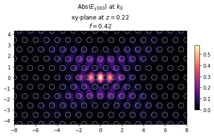
print("Cavity quality factor: %1.2f" %Q)

# We can also visualize the cavity and the mode profile of the fundamental mode
ax = legume.viz.field(gme, 'e', 0, Nx*Ny, z=dslab/2, component='y', val='abs', N1=300, N2=200)

Cavity quality factor: 6454.17

Autograd backend

Now the real fun starts. We can use legume and autograd to efficiently compute gradients of GME simulations. Let’s first define an objective function as the quality factor.

# To compute gradients, we need to set the `legume` backend to 'autograd'
legume.set_backend('autograd')

# Set GME options
gmax = 2
options = {'gmode_inds': [0], 'verbose': False, 'numeig': Nx*Ny+1, 'gradients': 'approx'}

# Define an objective function which is just the Q of the fundamental mode
def of_Q(params):
    dx = params[0:nc]
    dy = params[nc:]
    (gme, Q) = gme_cavity(dx, dy, gmax=gmax, options=options)

    # We put a negative sign because we use in-built methods to *minimize* the objective function
    return -Q

Test gradient of quality factor

We will test the legume gradient vs. a numerical check. Note that legume (through autograd) computes the gradients efficiently, using one backpropagation to get the derivative of the objective w.r.t. every parameter simultaneously. Because of time considerations, for the numerical finite-difference check we will only pick one parameter at random.

# The autograd function `value_and_grad` returns simultaneously the objective value and the gradient
obj_grad = value_and_grad(of_Q)

# We choose one parameter index at random for the numerical check
ind0 = np.random.randint(0, dx.size, 1)
# We set the starting parameters to zeros, i.e. un-modified cavity
pstart = np.zeros((2*nc, ))

# Compute the autograd gradients (NB: all at once!)
t = time.time()
grad_a = obj_grad(pstart)[1]
# Print the gradient w.r.t. the parameter index ind0
print("Autograd gradient:  %1.4f, computed in %1.4fs" %(grad_a[ind0], time.time() - t))

# Compute a numerical gradient for one selected index
t = time.time()
p_test = np.copy(pstart)
p_test[ind0] = p_test[ind0] + 1e-5
grad_n = (of_Q(p_test) - of_Q(pstart))/1e-5
print("Numerical gradient: %1.4f, computed in %1.4fs" %(grad_n, time.time() - t))

print("Relative difference: %1.2e" %np.abs((grad_a[ind0] - grad_n)/grad_n))

Autograd gradient:  -346.0501, computed in 14.3879s
Numerical gradient: -346.0546, computed in 13.8461s
Relative difference: 1.31e-05

The two gradients match very well, and the autograd simulation took as much time to get all the derivatives as it took the numerical simulation time to get just one of the derivatives. The magic of reverse-mode automatic differentiation!

Test gradient of fields

We will also illustrate computing the gradient with respect to an objective function that depends on the electric field of a mode. We define an objective function as the inverse of the maximum field intensity of the mode, which gives the mode volume (up to some constants). Note that in legume, fields are normalized to integrate to unity by definition.

# Define an objective function which is proportional to the V of the fundamental mode
def of_V(params):
    dx = params[0:nc]
    dy = params[nc:]
    (gme, Q) = gme_cavity(dx, dy, gmax=gmax, options=options)

    # Get the electric field in the center of the slab
    Ey = gme.get_field_xy('e', kind=0, mind=Nx*Ny, z=dslab/2, component='y', Nx=3, Ny=3)[0]['y']

    # Notice the use of autograd.numpy (npa) and not plain numpy (np)
    return 1/npa.square(npa.amax(npa.abs(Ey)))

# The autograd function `value_and_grad` returns simultaneously the objective value and the gradient
obj_grad = value_and_grad(of_V)

# We choose one parameter index at random for the numerical check
ind0 = np.random.randint(0, dx.size, 1)
# We set the starting parameters to zeros, i.e. un-modified cavity
pstart = np.zeros((2*nc, ))

# Compute the autograd gradients (NB: all at once!)
t = time.time()
grad_a = obj_grad(pstart)[1][ind0]
print("Autograd gradient:  %1.4f, computed in %1.4fs" %(grad_a, time.time() - t))

# Compute a numerical gradient for one selected index
t = time.time()
p_test = np.copy(pstart)
p_test[ind0] = p_test[ind0] + 1e-5
grad_n = (of_V(p_test) - of_V(pstart))/1e-5
print("Numerical gradient: %1.4f, computed in %1.4fs" %(grad_n, time.time() - t))

print("Relative difference: %1.2e" %np.abs((grad_a - grad_n)/grad_n))

//anaconda3/lib/python3.7/site-packages/numpy/core/numeric.py:538: ComplexWarning: Casting complex values to real discards the imaginary part
  return array(a, dtype, copy=False, order=order)

Autograd gradient:  0.0973, computed in 13.9638s
Numerical gradient: 0.0973, computed in 15.0929s
Relative difference: 8.39e-05

Note: the ComplexWarning comes from the way autograd implements np.dot(A, B) where A is real and B is complex. It can be disregarded, and as can be seen - the gradients are correct!

Quality factor optimization

The interesting thing about PhC cavities is that their Q can change dramatically upon small changes of the hole positions. On the other hand, the mode profile (and correspondingly the V) stay relatively unchanged. So, below we will optimize solely for the quality factor. Note that legume comes with a Minimize class that implements either adam or lbfgs minimization, which is what we are going to use. Of course, any external optimization function can also be combined with the gradient computation from legume.

# Set the objective function to be the quality factor
obj_grad = value_and_grad(of_Q)

# Initialize an optimization object; jac=True means that obj_grad returns both the value
# and the jacobian of the objective. The alternative syntax is Minimize(of, jac=grad_of)
opt = Minimize(obj_grad, jac=True)

# Starting parameters are the un-modified cavity
pstart = np.zeros((2*nc, ))

# Run an 'adam' optimization
(p_opt, ofs) = opt.adam(pstart, step_size=0.005, Nepochs=10, bounds = [-0.25, 0.25])

Epoch:    1/  10 | Duration:  13.35 secs | Objective: -6.454171e+03
Epoch:    2/  10 | Duration:  14.84 secs | Objective: -9.923204e+03
Epoch:    3/  10 | Duration:  15.49 secs | Objective: -1.613968e+04
Epoch:    4/  10 | Duration:  16.23 secs | Objective: -2.634551e+04
Epoch:    5/  10 | Duration:  15.59 secs | Objective: -3.837220e+04
Epoch:    6/  10 | Duration:  16.13 secs | Objective: -6.522058e+04
Epoch:    7/  10 | Duration:  15.64 secs | Objective: -9.175617e+04
Epoch:    8/  10 | Duration:  14.97 secs | Objective: -1.424175e+05
Epoch:    9/  10 | Duration:  14.68 secs | Objective: -2.015265e+05
Epoch:   10/  10 | Duration:  14.81 secs | Objective: -4.609714e+05

Note that the Q increased by almost two orders of magnitude in just 10 steps of the Adam optimization! Let’s visuzlize the optimized cavity below.

# Optimized parameters
dx = p_opt[0:nc]
dy = p_opt[nc:]

# Run the simulation
(gme, Q) = gme_cavity(dx, dy, gmax=gmax, options=options)
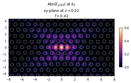
print("Cavity quality factor: %1.2f" %Q)
ax = legume.viz.field(gme, 'e', 0, Nx*Ny, z=dslab/2, component='y', val='abs', N1=200, N2=200)

Cavity quality factor: 460971.43

Refining the optimization

We note that we used a relatively fast optimization for illustration purposes. In the legume paper, we use gmax = 2.5, as well as a 3x3 \(k\)-grid in the Brillouin zone, and average the loss rates. This takes longer time to compute, and significantly more memory if done directly, because all the variables, including all the dense matrices and all the eigenvectors at every \(k\) are stored for the backpropagation. However, we provide a way to overcome this extra memory requirement at a low cost of computational time, as shown below.

First, we define a function that computes the loss rates over a specified set of \(k\)-points.

def gme_cavity_k(params, gmax, options, kpoints):
    dx = params[0:nc]
    dy = params[nc:]
    phc = cavity(dx, dy)
    options['compute_im'] = False
    gme = legume.GuidedModeExp(phc, gmax=gmax)
    gme.run(kpoints=kpoints, **options)
    fims = []
    for ik in range(kpoints[0, :].size):
        (freq_im, _, _) = gme.compute_rad(ik, [Nx*Ny])
        fims.append(freq_im)
    return (gme, npa.array(fims))

We can use this to compute the averaged \(Q\) in a straightforward way. Note that it’s better to average the loss rates and only then compute the \(Q\), rather than average the \(Q\)-s.

# Create an nkx x nky grid in k space (positive kx, ky only)
nkx = 3
nky = 3
kx = np.linspace(0, np.pi/Nx, nkx)
ky = np.linspace(0, np.pi/Ny/np.sqrt(3)*2, nky)
kxg, kyg = np.meshgrid(kx, ky)
kxg = kxg.ravel()
kyg = kyg.ravel()

def Q_kavg(params):
    (gme, fims) = gme_cavity_k(params, gmax, options, np.vstack((kxg, kyg)))
    # Note that the real part of the freq doesn't change much so we can just take ik=0 below
    return gme.freqs[0, Nx*Ny]/2/npa.mean(fims)

print("Refined cavity quality factor: %1.2f" %Q_kavg(p_opt))

Refined cavity quality factor: 41541.38

This \(Q\)-value is three times smaller than what we got above, and is likely closer to the true quality factor. For a converged optimization, it’s typically good to average over a small grid in \(k\)-space as shown here. To use this in an optimization, we can already use Q_kavg as an objective function, but, like mentioned above, this will require a lot of memory - specifically, about 9 times more than the original optimization at a single \(k\)-point. Here is how this can be overcome at a small cost of computational time.

# We set gmax=1 for this example to avoid memory issues
gmax = 1

# Objective function defining the average imaginary part
def fim_kavg(params):
    (gme, fims) = gme_cavity_k(params, gmax, options, np.vstack((kxg, kyg)))
    # Scale for easier printing
    return npa.mean(fims)*1e6

# Compute the gradient and time the computation; print just the first value
obj_grad = value_and_grad(fim_kavg)
t = time.time()
grad_a = obj_grad(pstart)[1]
print("Autograd gradient:  %1.4f, computed in %1.4fs" %(grad_a[0], time.time() - t))

Autograd gradient:  269.5663, computed in 22.0130s

Below is an altenative way to do the same thing; if you compare the memory usage between the cell below and the one above, you’ll realize the purpose of this whole thing.

We use a custom function that mimics map(lambda f: f(params), fns)) in a way that splits the gradient computation instead of storing all the intermediate variables for all functions. NB: the function fns all have to return a scalar and params are all vectors. fmap then returns an array of the same size as the number of functions in fns.

from legume.primitives import fmap

def of_kavg_fmap(params):
    # A function factory to make a list of functions for every k-point
    def fim_factory(ik):
        def fim(params):
            (gme, freq_im) = gme_cavity_k(params, gmax, options, np.array([[kxg[ik]], [kyg[ik]]]))
            return freq_im
        return fim

    fims = fmap([fim_factory(ik=ik) for ik in range(nkx*nky)], params)
    return npa.mean(fims)*1e6

# Compute the gradient and time the computation; print just the first value
obj_grad = value_and_grad(of_kavg_fmap)
t = time.time()
grad_a = obj_grad(pstart)[1]
print("Autograd gradient:  %1.4f, computed in %1.4fs" %(grad_a[0], time.time() - t))

Autograd gradient:  269.5663, computed in 26.9777s