Frequently Asked Questions
What do I do to test convergence?
The best way to make sure that your GME computation is converged is to increase the parameters controlling the precision of the simulation until you no longer see change in the eigenmodes of interest. We recommend doing this in the following order:
- First, make sure you have set a high enough
gmax, which is defined upon initialization ofGuidedModeExp. - Then, increase the number of guided bands included in the simulation by
adding more indexes to the
gmode_indslist supplied tolegume.GuidedModeExp.run(). Note that after including more modes ingmode_inds, you should test again the convergence w.r.t.gmax. - If your bands look particularly weird and discontinuous, there might be an
issue in the computation of the guided modes of the effective homogeneous
structure (the expansion basis). Try decreasing
gmode_stepsupplied inlegume.GuidedModeExp.run()to1e-3or1e-4and see if things look better.
Finally, note that GME is only an approximate method. So, even if the simulation is converged with respect to all of the above parameters but still produces strange results, it might just be that the method is not that well-suited for the structure you are simulating. We’re hoping to improve that in future version of legume!
Why am I running out of memory?
GME requrest the diagonalization of dense matrices, and you might start running
out of memory for simulations in which computational time is not that much of
an issue. This is also because the scaling with gmax is pretty bad: the
linear dimension of the matrix for diagonalization scales as gmax**2,
and so the total memory needed to store it scales as gmax**4. So,
unfortunately, if you’re running out of memory in a simulation there’s not much
you can do but decrease gmax.
That said, if you’re running out of memory in a gradient computation, there
could be something you can try. Reverse-mode autodiff is generally the best
approach for optimization problems in terms of computational time, but this can
sometimes come at a memory cost. This is because all of the intermediate
values of the forward simulation have to be stored for the backward pass.
So, if you are for example doing a loop through different k-points, the dense
matrices and their eigenvectors at every k will be stored, which can add up
to a lot. There is no easy way to fix this (and no direct way within
autograd), but we’ve included a function that can provide a workaround. For
details, have a look at this example.
Finally, it’s worth mentioning that there are probably improvements that can be made to the memory usage. If anybody wants to dive deep in the code and try to do that, it will be appreciated!
What should I know about the guided-mode basis?
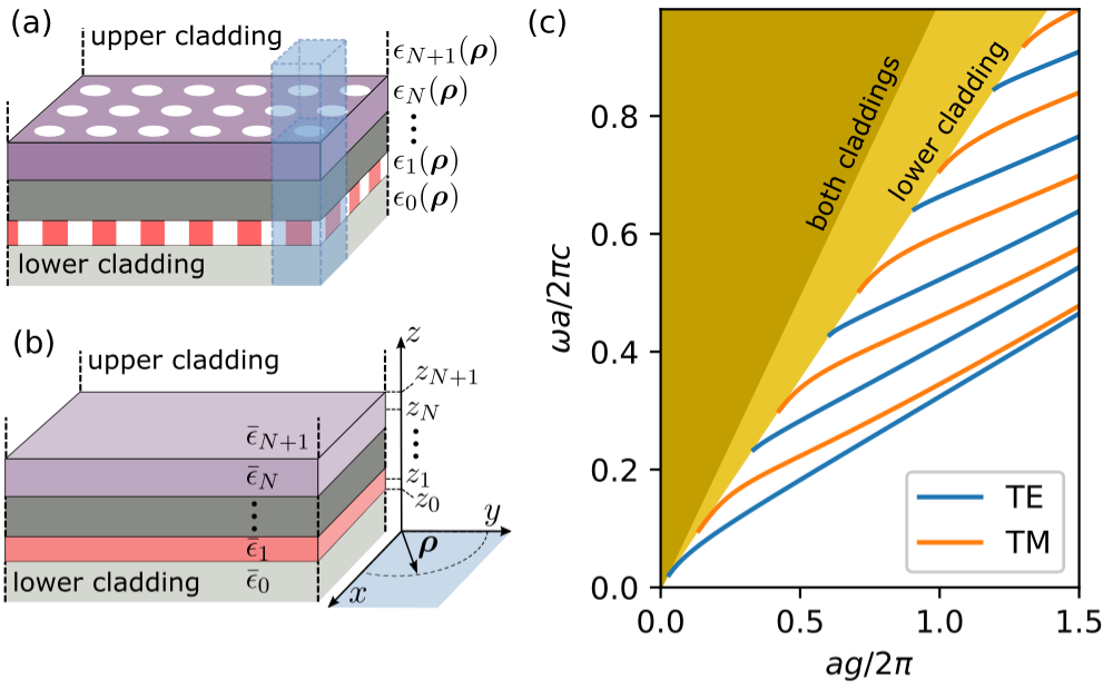
The expansion basis in the GME consists of the guided modes of an effective
homogeneous structure (panels (a)-(b)) in the Figure. By default, the
effective permittivities in (b) are taken as the average value in every layer.
This is controlled by the gmode_eps keyword option in the run options.
Setting gmode_eps = 'background' will take the background permittivity
instead, while there’s also the option to have custom values by setting
gmode_eps = 'custom'. In that case, every layer (including the claddings)
in the PhotCryst object should have a pre-defined effective permittivity
eps_eff, which will be used in the guided-mode computation. This is simply
set as an attribute of the layer, e.g.
phc.layers[0].eps_eff = 10   # Slab custom effective epsilon
phc.calddings[0].eps_eff = 1 # Lower cladding
phc.claddings[1].eps_eff = 5 # Upper cladding
The guided modes can be classified as TE/TM, where in our notation the reference
plane is the slab plane (xy). The guided modes alternate between TE and TM, such
that gmode_inds = [0, 2, 4, ...] are TE and gmode_inds = [1, 3, 5, ...]
are TM (panel (c)). However, this classification is often broken by the
photonic crystal structure (we discuss symmetries further below).
We only include the fully-guided modes in the computation (the ones that lie below both light lines in (c)). This is what makes the computation approximate, as the basis set is not complete.
How do I incorporate symmetry?
The TE/TM classification of the guided modes of the homogeneous structure is often broekn by the photonic crystal permittivity. Here is how you can still incorporate some structural symmetries.
For gratings (permittivity is periodic in one direction and homogeneous in the other), the TE/TM classification holds. You can selectively compute the modes by supplying gmode_inds with either only even or only odd numbers.
For photonic crystals with a mirror plane, like a single slab with symmetric
claddings, the correct classification of modes is with respect to reflection in
that plane. The positive-symmetry guided modes are
gmode_inds = [0, 3, 4, 7, 8, ...], while the negative-symmetry modes are
gmode_inds = [1, 2, 5, 6, 9, 10, ...]. Low-frequency positive-symmetry
modes that are mostly fromed by the gmode_inds = 0 guided band are
sometimes referred to as quasi-TE, and low-frequency negative-symmetry
modes that are mostly formed by the gmode_inds = 1 guided band are
sometimes referred to as quasi-TM.
Without any mirror planes, all the guided modes are generally mixed. There can still be symmetry if the k-vector points in a high-symmetry direction, but there is currently no way to take advantage of that in legume.
When should I use approximate gradients?
When running GME with the autograd backend, one of the run() options
you can specify is 'gradients' = {'exact' (default), 'approx'}. The
approximate option could be faster in some cases, and could actually still
be exact in some cases. This is the high-level computational graph of the
guided-mode expansion:
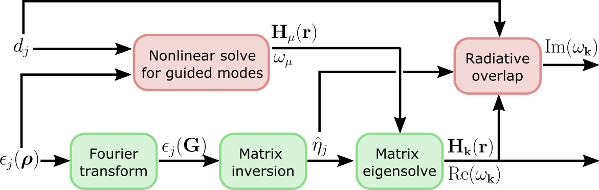
The 'approx' option discards the gradient due to the top path in this
graph, i.e. the gradient due to the changing basis. Only the gradient from the
diagonalization path is included. Here are some rules of thumb on what to use:
- If you’re optimizing hole positions, or more generally parameters that don’t
change the average permittivity, you’re in luck! In this case, the
'approx'gradients should actually be exact! - If you’re optimizing dispersion (real part of eigenfrequencies), you could try using
'approx'gradients, as they might be within just a few percent of the exact ones. - If you’re optimizing loss rates or field profiles
and/or if your parameters include the layer thicknesses, then the
'approx'gradients could be significantly off,'exact'is recommended (and is the default).
What if I only need the Q of some of the modes?
In some simulations, the computation of the radiative losses could be the time
bottleneck. In some cases, e.g. when optimizing a cavity, you only need to
compute the quality factor of a single mode. If you run the GME by default,
the Q-s of all modes will be computed instead, but you can set the option
compute_im = False to avoid this. Running the GME with this option will
compute all modes, but not the imaginary part of their frequencies (which is
done perturbatively after the first stage of the computation). Then, you can
use the legume.GuidedModeExp.compute_rad() method to only compute the loss rates
of selected modes.
What’s the gauge?
Something to be aware of is the fact that the eigenmodes come with an arbitrary k-dependent gauge, as is usually the case for eigenvalue simulations. That is to say, each eigenvector is defined only up to a global phase, and this phase might change discontinously even for nearby k-points. If you re looking into something that depends on the gauge choice, you will have to figure out how to set your preferred gauge yourself.
Of course, apart from this global phase, all the relative phases should be well-defined (as they correspond to physically observable quantities). So for example if you compute radiative couplings to S and P polarization, the relative phase between the two should be physical.
Can I speed things up if I need only a few eigenmodes?
The run options that can be supplied in legume.GuidedModeExp.run() include
numeig and eig_sigma, which define that numeig eigenmodes
closest to eig_sigma are to be computed. However, note that the default solver
defined by the eig_solver option is numpy.linalg.eigh, which always computes
all eigenvalues. Thus, numeig in this case only defines the number of
modes which will be stored, but it does not affect performance. If you’re
looking for a small number of eigenvalues, you can try setting eig_solver = eigsh,
which will use the scipy.sparse.linalg.eigsh method. In many cases this will
not be (much) faster, but it’s worth a try.
Note: using the eigsh solver when computing gradients comes with some
extra pros and cons. The added advantage is that the required memory should be lower,
because autograd does not need to store all the eigenvectors for the backward
pass (however, the matrices themselves are still stored, which could already
amount to a lot of memory). On the flip side, all the eigenvectors are needed
to compute exact gradients of any quantity that depends even on a single
eigenvector, so e.g. on loss rates or field profiles of the PhC eigenmodes. Thus,
the gradient of these quantities will be only approximate if computing only
a restricted number of eigenvectors (this does not apply to the eigh solver).
The gradients
could still be good enough for an optimization though, and, if the objective
function depends only on the frequencies of the PhC modes, then the gradients
should be exact.
How can I learn more about the method?
Our paper gives a lot of detail both on the guided-mode expansion method and on our differentiable implementation.
How should I cite legume?
If you find legume useful for your research, we would apprecite you citing our paper. For your convenience, you can use the following BibTex entry:
@article{Minkov2020,
title = {Inverse design of photonic crystals through automatic differentiation},
author = {Minkov, Momchil and Williamson, Ian A. D. and Gerace, Dario and Andreani, Lucio C. and Lou, Beicheng and Song, Alex Y. and Hughes, Tyler W. and Fan, Shanhui},
year = {2020},
journal = {arXiv:2003.00379},
}
Who made that awesome legume logo?
The legume logo was designed by Nadine Gilmer. She is also behind the logos for our angler and ceviche packages.