Bands of a photonic crystal slab

In this short example, we will demonstrate how Legume can be used to compute the bands of a photonic crystal slab. We will consider a slab design that is very close to one from the book Molding the Flow of Light.

First we will import the legume package:

import legume
import matplotlib.pyplot as plt

We will then define the parameters of our structure: \(D\) is the thickness of the slab, \(r\) is the radius of the air hole, and epsr is the permittivity.

D = 0.6
r = 0.3
epsr = 12.0

Next, we construct the lattice, the photonic crystal object, and the GME object:

lattice = legume.Lattice('hexagonal')
phc = legume.PhotCryst(lattice)
phc.add_layer(d=D, eps_b=epsr)
phc.layers[-1].add_shape(legume.Circle(eps=1.0, r=r))
gme = legume.GuidedModeExp(phc, gmax=6)

Warning: gmax=6 exactly equal to one of the g-vectors modulus, reciprocal lattice truncated with gmax=6.0000000001 to avoid problems.
Plane waves used in the expansion = 97.

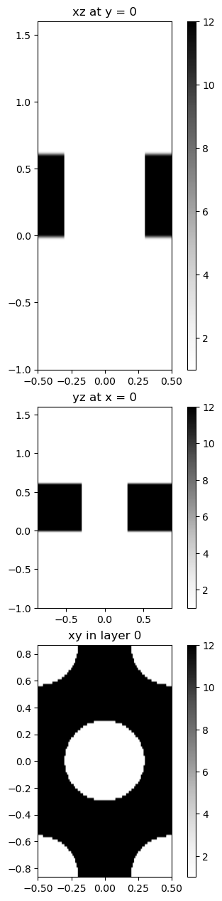
We can then use the legume.viz module to visualize our photonic crystal slab across three planes through the unit cell:

legume.viz.structure(phc, xz=True, yz=True, figsize=3.)

Finally, we can solve for the bands of the photonic crystal. Note that here we are solving for only the modes with TE-like polarization because we have gmode_inds=[0].

path = lattice.bz_path(['G', 'M', 'K', 'G'], [15, 10, 15])
gme.run(kpoints=path['kpoints'],
        gmode_inds=[0, 3],
        numeig=20,
        verbose=False)

Now the results are in the object gme and can be extracted with gme.freqs, gme.freqs_im, etc. Alternatively, we can plot the photonic bands directly with viz.bands. In the legume 1.0.0 version, viz.bands plots the frequencies as a function of wavevector along the path in the Brillouin zone by means of the kw argument k_units=True, which requires setting the xticks with path['k_indexes']. See documentation for details.

fig, ax = plt.subplots(1, figsize = (7, 5))
legume.viz.bands(gme, figsize=(5,5), k_units=True, Q=True, ax=ax)
ax.set_xticks(path['k_indexes'])
ax.set_xticklabels(path['labels'])
ax.xaxis.grid('True')

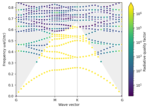
We observe excellent agreement with the bands shown in the text book (red lines).