Active metasurface simulation
In this notebook we show how to calculate the dispersion and properties of an active metasurface, i.e. sustaining an excitonic response. Excitons are electron-hole buond states that interact with light. If the interaction strength overcomes the photonic and excitonic losses, a new excited state is formed: the polariton. The theory of exciton-photon coupling leading to the formation to poalritons is developed in this paper.
[1]:
import legume
from legume import viz
import numpy as np
import copy
import matplotlib.pyplot as plt
print(f"legume version: {legume.__version__}")
legume version: 1.0.0
Photonic structure simulation
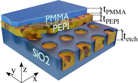
As an example, we take a pervoskite-based metasurfaced recently studied, see N.H.M. Dang et al., Advance Optical Materials (2020). It consist of a SiO\(_2\) core with etched air holes where a pervoskite material (PEPI) is inflitrated. The PEPI is the active material that sustains excitonic states. A residual PEPI layer lies on top of the etched region. Finally, the device is encapsulated with a polymer (PMMA) layer as depicted in the figure.
We start by defining the structure and calculating the purely photonic properties. We start by defining the main structural parameters.
[2]:
# lattice constant [nm]
a = 330
# Thicknesses of all layers
t_PMMA,t_PEPI,t_etch = 200/a, 30/a, 170/a
# Permettivity of all materials
eps_SiO2,eps_PEPI,eps_PMMA = 1.48**2,2.4**2 ,1.49**2
r = 0.2  # radius
gmax=6.1
In the first calculations round, we just the purely photonics properties. To do so, we initialize the photonic crystal slab.
[3]:
lattice_type = 'square'
lattice = legume.Lattice(lattice_type)

phc = legume.PhotCryst(lattice,eps_l=eps_SiO2)

phc.add_layer(d=t_etch, eps_b=eps_SiO2)
phc.add_layer(d=t_PEPI, eps_b=eps_PEPI)
phc.add_layer(d=t_PMMA, eps_b=eps_PMMA)

phc.layers[-3].add_shape(legume.Circle(eps=eps_PEPI, r=r))
To better compare with experimental data, we calculate the dispersion in the same wavevector range as in the paper: \(k\in[-4,4]\mu\text{m}^{-1}\). In legume notation, wavevectors are in units of \(k_{\text{leg}}=ka\), with \(k\) and \(a\) the wavevector and the lattice constant in [m]
[4]:
k_dim_max = 4 # um^-1
k_max = k_dim_max*a/1000   # Dimensionless maximum wavevector
num_k = 30
path = lattice.bz_path([[-k_max,1e-15],"G",[k_max,0]],[num_k])
gme_options = {'gmode_inds':[0,1,2,3],
        'numeig':8,
        'verbose':True}
gme = legume.GuidedModeExp(phc,gmax=gmax)
gme.run(kpoints=path['kpoints'],**gme_options)
Running gme k-points: │██████████████████████████████│ 61 of 61
┏━━━━━━━━━━━━━━━━━━━━━━━━━━━━━━━━━━━━━━━━━━━━━━━━━━━━━━━━━━━━┳━━━━━━━━━━┳━━━━━━━━━━━━━━━━━━━━━━━━━━━━━━┓
┃ Steps in GuidedModeExp: 121 plane waves and 4 guided modes ┃ Time (s) ┃                 % vs total T ┃
┡━━━━━━━━━━━━━━━━━━━━━━━━━━━━━━━━━━━━━━━━━━━━━━━━━━━━━━━━━━━━╇━━━━━━━━━━╇━━━━━━━━━━━━━━━━━━━━━━━━━━━━━━┩
│ Guided modes computation with gmode_compute='exact'        │ 15.369   │ │████████████--------│   63% │
│ Inverse matrix of Fourier-space permittivity               │ 0.002    │ │--------------------│    0% │
│ Matrix diagionalization using the 'eigh' solver            │ 1.678    │ │█-------------------│    7% │
│ Creating GME matrix                                        │ 7.448    │ │██████--------------│   30% │
├────────────────────────────────────────────────────────────┼──────────┼──────────────────────────────┤
│ Total time for real part of frequencies for 61 k-points    │ 24.529   │ │████████████████████│  100% │
└────────────────────────────────────────────────────────────┴──────────┴──────────────────────────────┘
Running GME losses k-point: │██████████████████████████████│ 61 of 61
┏━━━━━━━━━━━━━━━━━━━━━━━━━━━━━━━━━━━━━━━━━━━━━━━━━━━━━━━━━━━━━━━━━┳━━━━━━━━━━┓
┃ Steps in GuidedModeExp: 121 plane waves and 4 guided modes      ┃ Time (s) ┃
┡━━━━━━━━━━━━━━━━━━━━━━━━━━━━━━━━━━━━━━━━━━━━━━━━━━━━━━━━━━━━━━━━━╇━━━━━━━━━━┩
│ Total time for imaginary part of frequencies for 488 eigenmodes │ 5.032    │
└─────────────────────────────────────────────────────────────────┴──────────┘
[5]:
fig, ax = plt.subplots(1, figsize = (4, 3.5))
legume.viz.bands(gme,ax=ax,a=a*1e-9,eV=True)
ax.set_xticks(path['indexes'])
ax.set_xticklabels([f"{k_dim_max}","0",f"{k_dim_max}"])
ax.set_xlabel("Wavector ($\\mu$m$^{-1}$)")
ax.set_ylim(2,2.6)
[5]:
(2.0, 2.6)
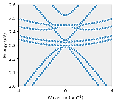
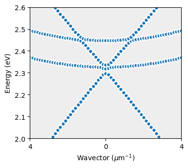
These bands won’t compare well with experimental data since the the excitation light is s-(TE) polarized. For a direct comparison, we recalculate only the odd modes with respect the vertical plane of symmetry. Under the diffraction limit, these modes correspond to the one excited by an s-polarized pump.
[6]:
gme_options = {'gmode_inds':[0,1,2,3],
        'numeig':8,
        'verbose':True,
        'kz_symmetry': "odd",
        'angles':path['angles']}
gme.run(kpoints=path['kpoints'],**gme_options)
Running gme k-points: │██████████████████████████████│ 61 of 61
┏━━━━━━━━━━━━━━━━━━━━━━━━━━━━━━━━━━━━━━━━━━━━━━━━━━━━━━━━━━━━┳━━━━━━━━━━┳━━━━━━━━━━━━━━━━━━━━━━━━━━━━━━┓
┃ Steps in GuidedModeExp: 121 plane waves and 4 guided modes ┃ Time (s) ┃                 % vs total T ┃
┡━━━━━━━━━━━━━━━━━━━━━━━━━━━━━━━━━━━━━━━━━━━━━━━━━━━━━━━━━━━━╇━━━━━━━━━━╇━━━━━━━━━━━━━━━━━━━━━━━━━━━━━━┩
│ Guided modes computation with gmode_compute='exact'        │ 15.364   │ │████████████--------│   63% │
│ Inverse matrix of Fourier-space permittivity               │ 0.000    │ │--------------------│    0% │
│ Matrix diagionalization using the 'eigh' solver            │ 0.395    │ │--------------------│    2% │
│ Creating GME matrix                                        │ 7.160    │ │█████---------------│   30% │
│ Creating change of basis matrix using dense matrices       │ 1.243    │ │█-------------------│    5% │
├────────────────────────────────────────────────────────────┼──────────┼──────────────────────────────┤
│ Total time for real part of frequencies for 61 k-points    │ 24.201   │ │████████████████████│  100% │
└────────────────────────────────────────────────────────────┴──────────┴──────────────────────────────┘
Running GME losses k-point: │██████████████████████████████│ 61 of 61
┏━━━━━━━━━━━━━━━━━━━━━━━━━━━━━━━━━━━━━━━━━━━━━━━━━━━━━━━━━━━━━━━━━┳━━━━━━━━━━┓
┃ Steps in GuidedModeExp: 121 plane waves and 4 guided modes      ┃ Time (s) ┃
┡━━━━━━━━━━━━━━━━━━━━━━━━━━━━━━━━━━━━━━━━━━━━━━━━━━━━━━━━━━━━━━━━━╇━━━━━━━━━━┩
│ Total time for imaginary part of frequencies for 488 eigenmodes │ 5.930    │
└─────────────────────────────────────────────────────────────────┴──────────┘
[7]:
fig, ax = plt.subplots(1, figsize = (4, 3.5))
legume.viz.bands(gme,ax=ax,a=a*1e-9,eV=True)
ax.set_xticks(path['indexes'])
ax.set_xticklabels([f"{k_dim_max}","0",f"{k_dim_max}"])
ax.set_xlabel("Wavector ($\\mu$m$^{-1}$)")
ax.set_ylim(2,2.6)
[7]:
(2.0, 2.6)
Excitons in legume
Before delving into polaritonic simulations, it’s essential to understand the foundational concept of excitons within the Legume code. Excitons are quasiparticles formed by bound electron-hole states. The binding energy of excitons can be notably influenced in systems where excitons experience confinement along a specific direction. Examples of such systems include semiconductor quantum wells, perovskites, or monolayers of transition metal dichalcogenides.
In the context of legume, excitons are treated as being perfectly confined within a 2D plane. The dynamics of excitons are calculated by solving the 2D Schrödinger equation. Analogous to how photons in periodically patterned Photonic Crystals (PhCs) feel a periodic potential, excitons also experience a periodic potential when the 2D layer is patterned. For instance, holes etched in a quantum well layer act as barriers for the excitonic wavefunction. Conversely, a pillar of perovskite
provides a potential well where excitons can exist. This potential alters the dispersion relation and the wavefunction of free excitons.
Setting up ExcitonSchroedEq Simulation
To investigate the impact of a potential on excitonic eigenmodes, we initiate an ExcitonSchroedEq simulation. We start by defining some excitonic parameters: the bare exciton energy \(E_0\) epressed in eV, the excitonic mass \(M\) in kg and the non-radiative losses of excitons loss in eV. For the mass, we can take a fraction of the free electron mass \(m_e\) from legume.constant module.
[8]:
M = legume.constants.m_e*0.2
E0 = 2.394
loss = 5*10**-4 #[eV]
Before running the simulation, we have to specify few other parameters. Firsst of all, the z-position, determining the location of the 2D simulation. This will define the layer of the phc from which we ShapesLayer objects are taken, subsequently characterizing the in-plane potential. Each of these ShapesLayer objects is associated with a potential V_shapes with respect to a background at null potential. In the present example, we want to simulate PEPI pillars where excitons
can dwell. Consequently, a negative (attractive) potential, V_shapes=-1, is configured to appropriately model this scenario.
[9]:
exc_options = {'numeig_ex':8,
        'verbose_ex':True}
V = -1 # Negative potential for PEPI pillars
z = phc.layers[0].z_mid # center of the layer with pillar
exc_pill = legume.ExcitonSchroedEq(phc,z=z,V_shapes=V,a=a,M=M,E0=E0,loss= loss,\
                                gmax=gmax,truncate_g='abs')
exc_pill.run(kpoints=path["kpoints"], **exc_options)
Running ESE k-point: │------------------------------│ 2 of 61Running ESE k-point: │██████████████████████████████│ 61 of 61
┏━━━━━━━━━━━━━━━━━━━━━━━━━━━━━━━━━━━━━━━━━━━━━━━━━━━┳━━━━━━━━━━┳━━━━━━━━━━━━━━┓
┃ Steps in ExcitonSchroedEq: 121 plane waves        ┃ Time (s) ┃ % vs total T ┃
┡━━━━━━━━━━━━━━━━━━━━━━━━━━━━━━━━━━━━━━━━━━━━━━━━━━━╇━━━━━━━━━━╇━━━━━━━━━━━━━━┩
│ Diagonalization of the Hamiltonian                │ 0.0819   │          62% │
├───────────────────────────────────────────────────┼──────────┼──────────────┤
│ Total time for excitonic energies for 61 k-points │ 0.1328   │         100% │
└───────────────────────────────────────────────────┴──────────┴──────────────┘
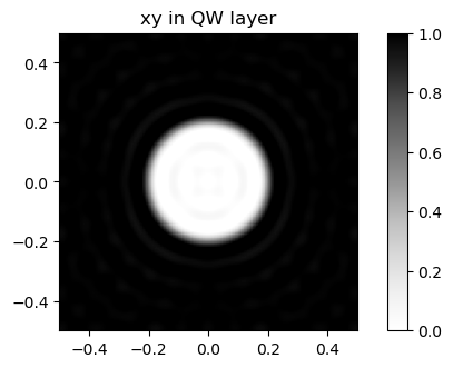
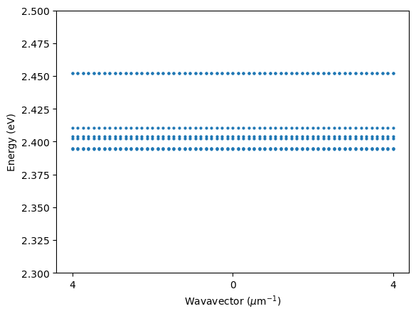
We can begin by examining the real-space potential derived from the Fourier components employed in the computation, along with exploring the quantized excitonic bands. These bands are very flattened indicating excitonic modes extremely confined in the pillars.
[10]:
legume.viz.pot_ft(exc_pill)
plt.show()
fig,ax = plt.subplots()
for ind,e in enumerate(exc_pill.eners):
        ax.scatter([ind]*8,np.real(e) ,c="C0",s=4 )
ax.set_xticks(path['indexes'])
ax.set_xticklabels([f"{k_dim_max}","0",f"{k_dim_max}"])
ax.set_xlabel("Wavavector ($\\mu$m$^{-1}$)")
ax.set_ylabel("Energy (eV)")
ax.set_ylim(2.3,2.5)
plt.show()
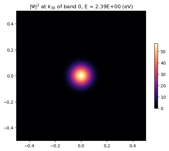
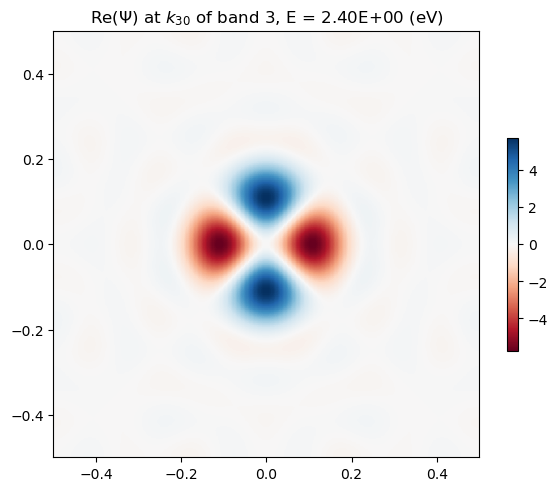
Finally, we can exploit viz.wavef to plot the wavefunction of modes. Specifically, we plot the wavefunctions associated with the lowest and fourth bands.
[11]:
plot1 = legume.viz.wavef(exc_pill,
    kind=num_k,
    mind=0,
    val="abs2",
    cbar=True,)
plot2= legume.viz.wavef(exc_pill,
    kind=num_k,
    mind=3,
    val="re",
    cbar=True,)
Polaritonic simulation
So far, we’ve computed the photonic and excitonic properties separately. Now, it’s time to turn on light-matter interaction! Everything is handled by legume, all we need to do is to add 2D active layers to the PhotCryst. We can do that with the add_qw method. Additionally to what we did with the ExcitonSchroedEq simulation, here we have to provide the vecotrial oscillator strength in the excitonic resonance in the \([x,y,z]\) frame of reference. For each \(z\)-position,
we place two active well layers with either purely \(\hat{x}\)- and \(\hat{y}\)-polarized.
[12]:
osc_str_x = 2*10**19*np.array([1,0,0]) # Oscillator strength per unit per unit surface [m^-2]
osc_str_y = 2*10**19*np.array([0,1,0])

# Biuld the PhC
phc = legume.PhotCryst(lattice,eps_l=eps_SiO2)
phc.add_layer(d=t_etch, eps_b=eps_SiO2)
phc.add_layer(d=t_PEPI, eps_b=eps_PEPI)
phc.add_layer(d=t_PMMA, eps_b=eps_PMMA)
phc.layers[0].add_shape(legume.Circle(eps=eps_PEPI, r=r))

# Add active layers
phc.add_qw(z=phc.layers[0].z_mid,V_shapes=-1,a=a*1e-9,M=M,E0=E0,loss=loss,\
                                osc_str=osc_str_x)
phc.add_qw(z=phc.layers[0].z_mid,V_shapes=-1,a=a*1e-9,M=M,E0=E0,loss= loss,\
                                osc_str=osc_str_y)
phc.add_qw(z=phc.layers[1].z_mid,V_shapes=-1,a=a*1e-9,M=M,E0=E0,loss= loss,\
                                osc_str=osc_str_x)
phc.add_qw(z=phc.layers[1].z_mid,V_shapes=-1,a=a*1e-9,M=M,E0=E0,loss= loss,\
                                osc_str=osc_str_y)
[13]:
exc_options["verbose_ex"] = False
pol = legume.HopfieldPol(phc,gmax)
pol.run(kpoints=path['kpoints'],gme_options=gme_options,exc_options=exc_options)
Running gme k-points: │██████████████████████████████│ 61 of 61
┏━━━━━━━━━━━━━━━━━━━━━━━━━━━━━━━━━━━━━━━━━━━━━━━━━━━━━━━━━━━━┳━━━━━━━━━━┳━━━━━━━━━━━━━━━━━━━━━━━━━━━━━━┓
┃ Steps in GuidedModeExp: 121 plane waves and 4 guided modes ┃ Time (s) ┃                 % vs total T ┃
┡━━━━━━━━━━━━━━━━━━━━━━━━━━━━━━━━━━━━━━━━━━━━━━━━━━━━━━━━━━━━╇━━━━━━━━━━╇━━━━━━━━━━━━━━━━━━━━━━━━━━━━━━┩
│ Guided modes computation with gmode_compute='exact'        │ 15.137   │ │████████████--------│   64% │
│ Inverse matrix of Fourier-space permittivity               │ 0.001    │ │--------------------│    0% │
│ Matrix diagionalization using the 'eigh' solver            │ 0.381    │ │--------------------│    2% │
│ Creating GME matrix                                        │ 7.065    │ │█████---------------│   30% │
│ Creating change of basis matrix using dense matrices       │ 1.218    │ │█-------------------│    5% │
├────────────────────────────────────────────────────────────┼──────────┼──────────────────────────────┤
│ Total time for real part of frequencies for 61 k-points    │ 23.836   │ │████████████████████│  100% │
└────────────────────────────────────────────────────────────┴──────────┴──────────────────────────────┘
Running GME losses k-point: │██████████████████████████████│ 61 of 61
┏━━━━━━━━━━━━━━━━━━━━━━━━━━━━━━━━━━━━━━━━━━━━━━━━━━━━━━━━━━━━━━━━━┳━━━━━━━━━━┓
┃ Steps in GuidedModeExp: 121 plane waves and 4 guided modes      ┃ Time (s) ┃
┡━━━━━━━━━━━━━━━━━━━━━━━━━━━━━━━━━━━━━━━━━━━━━━━━━━━━━━━━━━━━━━━━━╇━━━━━━━━━━┩
│ Total time for imaginary part of frequencies for 488 eigenmodes │ 5.897    │
└─────────────────────────────────────────────────────────────────┴──────────┘
Running HP k-points: │██████████████████████████████│ 61 of 61
┏━━━━━━━━━━━━━━━━━━━━━━━━━━━━━━━━━━━━━━━━━━━━━━━━━━━━━━━━━━━━━━━━━━━━━━━━━━━━━━━━┳━━━━━━━━━━┓
┃ Steps in HopfieldPol: 8 photonic modes, 4 active layers with 8 excitonic modes ┃ Time (s) ┃
┡━━━━━━━━━━━━━━━━━━━━━━━━━━━━━━━━━━━━━━━━━━━━━━━━━━━━━━━━━━━━━━━━━━━━━━━━━━━━━━━━╇━━━━━━━━━━┩
│ Total time for matrix calculation and diagonalization for 61 k-points          │ 4.7937   │
└────────────────────────────────────────────────────────────────────────────────┴──────────┘
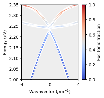
Finally, we can plot the polaritonic bands with viz.pol_bands, where the excitonic fraction is encoded with a colorscale. Blue modes correspond to mostly photonic modes, on the contrary reddish modes correspond to moslty excitonic polaritons.
[14]:
fig, ax = plt.subplots(1, figsize = (3, 3.2))
legume.viz.pol_bands(pol,fraction=True,ax=ax)
ax.set_xticks(path['indexes'])
ax.set_xticklabels([f"{-k_dim_max}","0",f"{k_dim_max}"])
ax.set_xlabel("Wavavector ($\\mu$m$^{-1}$)")
plt.ylim(2.,2.35)
[14]:
(2.0, 2.35)